

For most of modern economic history, explanations have focused on institutions, geography, culture, and historical contingency. Some countries developed more capable states, some were better positioned for trade, some accumulated technical knowledge earlier, and some experienced wars or political shocks that permanently changed their paths. Those explanations remain central.
There is also a narrower possibility that economists rarely put into cross-country growth models: populations may differ slightly, on average, in inherited traits related to learning and human-capital accumulation. That does not mean genes determine the destiny of countries. Development depends on policy, health, migration, institutions, incentives, conflict, and chance. The question is whether education-linked genetic differences contribute any predictive information once some of that history is taken into account.
I tested that question in 38 countries with genetic estimates and comparable economic data from 1970 to 2019.
Why growth is a harder test than wealth
The genetic evidence begins with a genome-wide association study, usually shortened to GWAS. A GWAS scans genetic variants in a large sample and asks whether each variant is statistically associated with a trait. Here the trait is educational attainment—roughly, years of schooling completed. Each individual association is tiny, uncertain, and not usefully interpreted on its own.
A polygenic score, or PGS, combines many of those small estimated associations into one index. For each sampled population, I multiplied the education-GWAS weight at each variant by its estimated frequency and added the results. A PGS is a statistical predictor, not an education gene, a measure of human value, or a fixed forecast of anyone’s life. Its meaning is especially indirect when it is averaged across population samples and assigned to a country.
I used two published scores. EA3 comes from the 2018 study led by James Lee, which analyzed about 1.1 million people. EA4 is the 2022 successor led by Aysu Okbay, based on roughly 3 million people and including within-family analyses. I standardized EA3 and EA4 across the final country sample, averaged them equally, and standardized the average again. Equal weighting is simple and transparent. It also avoids pretending that the two studies are independent replications, because some participants and much of the underlying genetic signal overlap.
The outcome is not how rich a country is today. It is average annual growth in real GDP per person between 1970 and 2019: the change in log GDP per person, divided by 49 years and expressed as a percentage. In ordinary language, this measures how quickly each country’s average income rose over the period.
The first look at the data
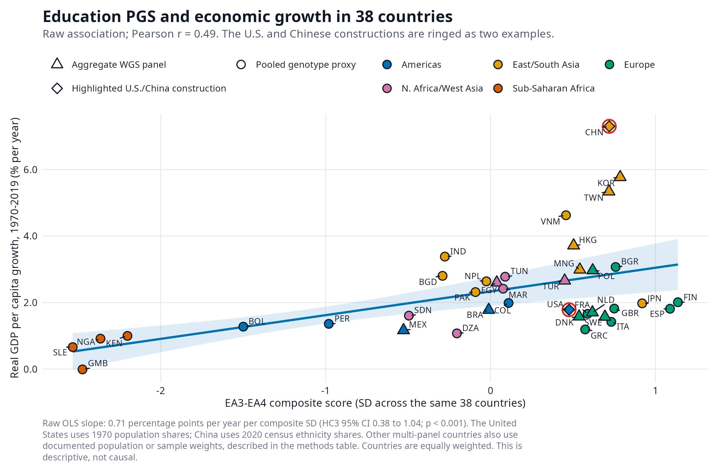
The unadjusted pattern is positive. Across the 38 countries, the Pearson correlation between the composite score and annual real-GDP-per-person growth is 0.49. In a simple regression, a one-standard-deviation higher score is associated with 0.71 percentage points faster annual growth. The 95% uncertainty interval runs from 0.38 to 1.04 percentage points. Figure 1 shows the individual countries behind that line.
Figure 1. Raw education-PGS composite and 1970–2019 annual growth in real GDP per person across 38 countries.
Accounting for where countries started
The raw relationship is not the most informative test. Countries did not start 1970 at the same level of development. Poorer countries can often grow quickly by adopting machinery, knowledge, and organizational practices already used elsewhere. Economists call this convergence. Rich countries usually have less room for that kind of easy catch-up.
I therefore control for GDP per person in 1970. The comparison becomes: among countries beginning at roughly similar income levels, did the country with the higher education-linked score subsequently grow faster?
In this conditional-convergence model, the estimated association is 1.16 percentage points per score standard deviation, with a 95% interval from 0.76 to 1.57.
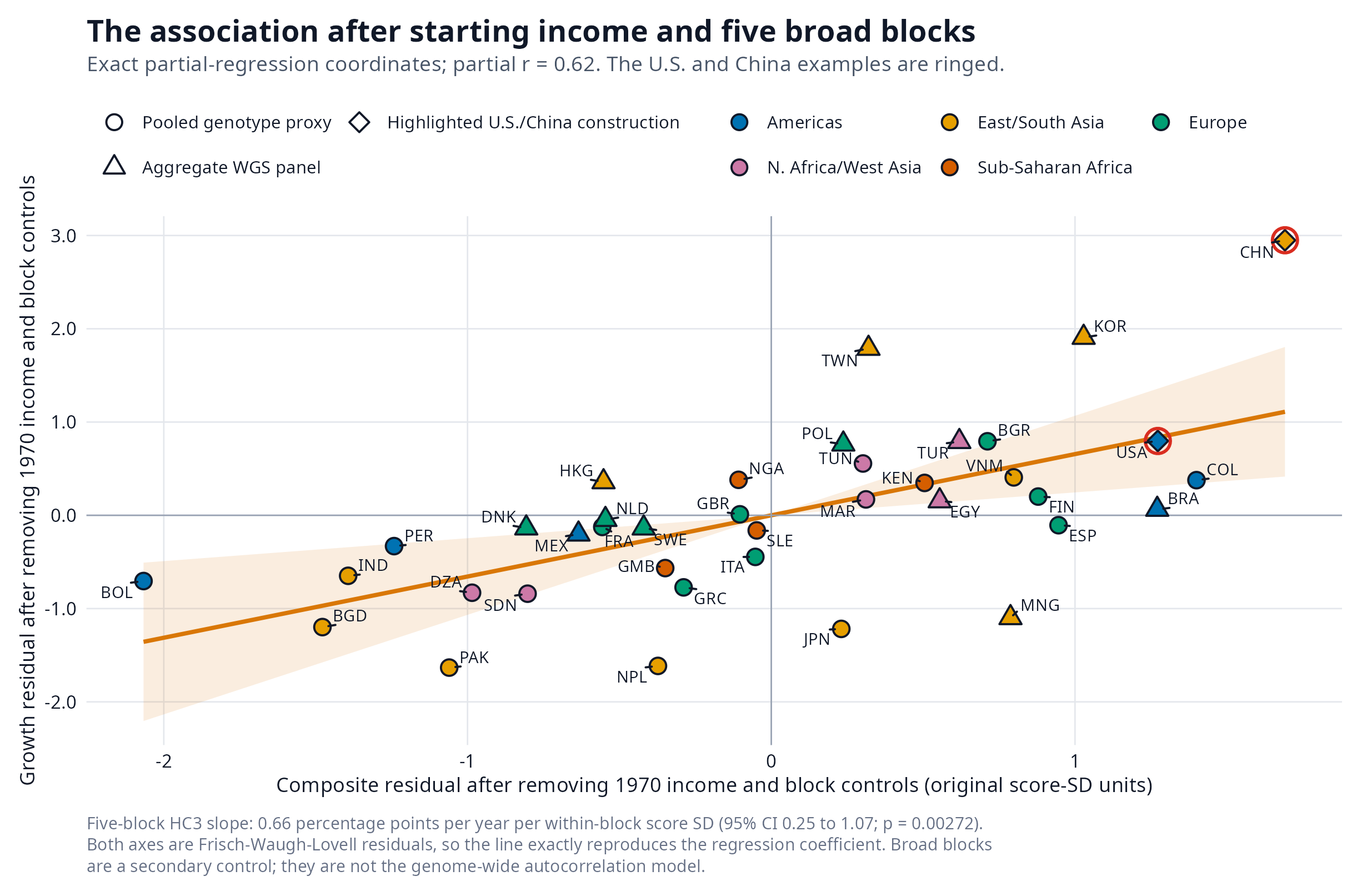
A simpler ancestry correction adds five broad ancestry-geography blocks. Its estimate is 0.66 percentage points, with a 95% interval from 0.25 to 1.07. Figure 2 introduces this adjusted relationship before any more elaborate genetic model: both axes remove starting-income and five-block differences. It is useful as an intuitive comparison, but broad categories cannot capture the fine-grained relatedness among populations.
Figure 2. Relationship after removing 1970 income and five broad ancestry-geography blocks from both axes.
Using the rest of the genome as a control
The hardest objection is genetic autocorrelation. Countries are not independent genetic units. Nearby and historically connected populations tend to resemble one another across the genome. They may also share institutions, migration histories, languages, and exposure to regional shocks. An education-PGS association could therefore be a disguised ancestry or history association.
The main robustness test uses 2,959 LD-pruned markers spread across the genome, with the education-score loci excluded. From their allele frequencies I constructed a country-by-country relatedness matrix. The model then allows the unexplained growth outcomes of genetically similar countries to be correlated. Instead of deciding that all members of a continent are equivalent, it uses the full pairwise pattern of genome-wide similarity.
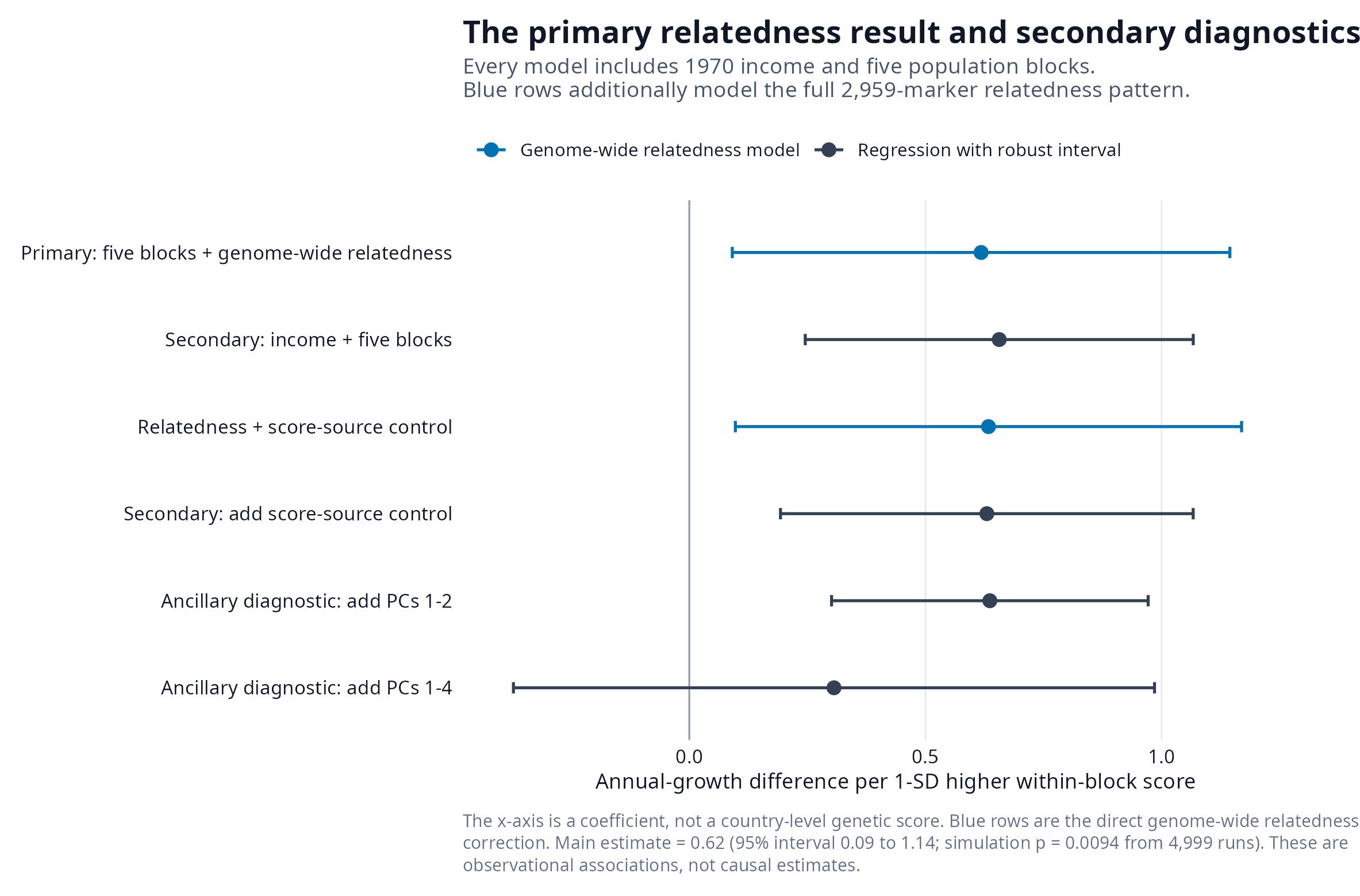
In this genome-wide relatedness model, a one-standard-deviation higher within-block composite is associated with 0.62 percentage points faster annual growth in real GDP per person. The conditional 95% interval runs from 0.09 to 1.14. In 4,999 datasets simulated under a null model with no score effect, a result this strong appeared about 0.9% of the time.
That simulation is a demanding check, but it is not magic. It treats the country scores, allele frequencies, and relatedness matrix as known rather than propagating every layer of sampling error. It also cannot remove an omitted historical factor simply because that factor is correlated with ancestry in a complicated way. Figure 3 compares the main relatedness result with the five-block estimate and ancillary specifications. Its horizontal axis is the estimated association with annual growth, not a country-level genetic-similarity score.
Figure 3. Estimated annual-growth association across model specifications.
How a national genetic score is constructed
Turning population panels into national averages is an important limitation, not a clerical detail. A panel carrying a country label is rarely a random sample of the whole country. Whenever several identifiable groups represent a country and defensible demographic information exists, I weight the represented groups by documented population shares. When the available groups cover only part of the population, the primary rule normalizes their shares within that covered portion; where a broad residual proxy exists, it represents the documented remainder. The identical weights are used for the PGS and the genome-wide marker frequencies. The full component weights, coverage shares, sources, and sensitivity rules are preserved in the accompanying methods CSV.
The United States and China illustrate the approach. For the United States, the primary construction uses 1970 population shares and three imperfect genetic proxies: CEU for non-Hispanic White residents, ASW for non-Hispanic Black residents, and MXL for Hispanic or Latino residents. Those categories cover 98.82% of the 1970 population; within the represented share, their weights are 84.47%, 11.01%, and 4.52%, respectively.
For China, Han populations receive the overwhelming majority of the weight: the census Han share is 91.11%. Several Han panels are first combined into the Han component, while sampled minority panels receive their documented shares and the remaining unsampled minority share follows the stated residual rule. Across the five matched U.S. demographic scenarios, the main relatedness-model coefficient ranges from 0.59 to 0.62 percentage points.
These are still approximations. Census race and ethnicity are social self-identifications, not genetic ancestries. CEU, ASW, MXL, and the Chinese panels are narrow samples, not miniature national censuses. The same caveat applies elsewhere, even after demographic reweighting. A carefully documented national proxy is better than silently giving every available panel equal weight, but it does not become a probability sample.
What the secondary checks say
The five-block model is a readable secondary check; the genome-wide matrix is the main one. I also report principal-component specifications only as ancillary diagnostics. Principal components compress major axes of genetic variation into a few variables, but here they can remove variation in the education score itself as well as unrelated structure. With two PCs the estimate is 0.64; with four it is 0.31 percentage points. These results show sensitivity to how ancestry is parameterized, but I do not treat the PC models as more authoritative than the full relatedness model.
No single country determines the sign. Re-estimating the main model after omitting each country in turn leaves the coefficient between 0.41 and 0.68 percentage points. Every leave-one-out estimate remains positive. Yet the uncertainty interval crosses zero in 19 of the 38 runs; the estimate falls most when United States or Brazil is omitted. That check can detect a spectacularly influential country; it cannot detect a bias shared across many countries.
Catch-up, innovation, and institutions
A correlation is more informative when its pattern matches a plausible mechanism. Education-linked traits might matter most in poorer countries if they help populations absorb existing technologies. That is the technological catch-up hypothesis. Alternatively, they might matter most near the frontier, where growth depends more on research, entrepreneurship, and creating new technology.
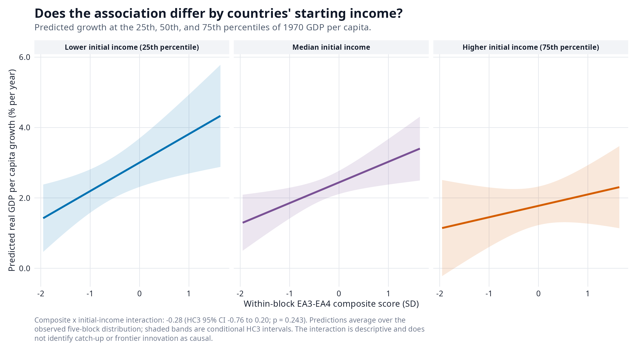
I tested this by interacting the score with 1970 income. The interaction is negative at −0.28 percentage points, with a 95% interval from −0.76 to 0.20. Its sign leans toward a catch-up interpretation, in which the association is stronger among initially poorer countries. The interval includes zero, so the data do not clearly distinguish the two mechanisms. Figure 4 shows predicted growth across score values for countries at lower, median, and higher starting-income levels.
A second interaction asks whether stronger initial institutions let education-linked traits produce larger economic returns. Its estimate is −0.26 percentage points, with a 95% interval from −0.67 to 0.15. The interval includes zero, so this sample provides no clear evidence that the association is stronger under better institutions. With only this many countries, both interaction tests are imprecise and should be read as clues about mechanism rather than decisive findings.
Figure 4. Predicted annual real-GDP-per-person growth across education-PGS values at lower, median, and higher 1970 income.
Conclusion
The narrow result is that countries with higher EA PGS tended to experience faster annual growth in real GDP per person from 1970 to 2019. The association survives adjustment for starting income and a model in which genome-wide relatedness shapes the covariance of unexplained growth.
Sources and further reading
Lee, J.J., Wedow, R., Okbay, A. et al. (2018). Gene discovery and polygenic prediction from a genome-wide association study of educational attainment in 1.1 million individuals. Nature Genetics, 50, 1112-1121. https://doi.org/10.1038/s41588-018-0147-3
Okbay, A., Wu, Y., Wang, N. et al. (2022). Polygenic prediction of educational attainment within and between families from genome-wide association analyses in 3 million individuals. Nature Genetics, 54, 437-449. https://doi.org/10.1038/s41588-022-01016-z
The 1000 Genomes Project Consortium. (2015). A global reference for human genetic variation. Nature, 526, 68-74. https://doi.org/10.1038/nature15393
Feenstra, R.C., Inklaar, R. & Timmer, M.P. (2015). The Next Generation of the Penn World Table. American Economic Review, 105(10), 3150-3182. https://doi.org/10.1257/aer.20130954
Great analysis and conclusion.
"Can Genes Help Countries Get Rich?"
I believe there are genetically controlled or influenced human traits that can facilitate a nation's wealth. But the question is, what is the distribution of value to the populace?